GMN+: A Binary Homologous Vulnerability Detection Method Based on Graph Matching Neural Network with Enhanced Attention

Intro

It is safe to say that there are a lot of vulnerable applications out there. Unfortunately, many of these vulnerabilities are hard to detect. The difficulty can be attributed to the fact that modern software is incredibly complex with a lot of moving parts. Because of this complexity, there is a heavy push for code reuse, which in turn can lead to introducing the same vulnerability in multiple codebases. These kinds of vulnerabilities are called Homologous Vulnerabilities, and in the following text, I am going to introduce you to a State of the Art approach for detecting these kinds of vulnerabilities with a mixture of BERT like embedding models and Graph Neural Networks (GNN). This combination is very widespread in vulnerability detection research and I compiled an overview of possible approaches for LLM-GNN merge here. But without further ado, let’s start with GMN+.

GMN+

What does GMN mean? It is an acronym for Graph Matching (Neural) Network, which is a Deep Neural Network that tries to map nodes from one graph to nodes of the second graph by learning similarities and patterns between the two graphs. The main reason why we use Neural Networks or formulate Graph Matching as a prediction problem is to make it tractable (find an approximate solution), since the problem of determining similarities or shared patterns between two graphs is NP hard.

High Level Idea

GMN+ works on a function level, this means that we are going to construct a graph for every function. Functions are extracted directly from binary code using a disassembler. Individual nodes of a graph are further preprocessed and at the end we always take a pair of functions and determine if they are homologous or not by comparing the information within a function and between the two functions.

Method

We can break down the High Level idea into 3 parts:

Instruction Preprocessor
Semantic Learner
Graph Learner

Instruction Preprocessor

The Instruction Preprocessor takes a binary and disassembles its instructions and set of functions. The disassembly is performed with IDA Pro, where each function is split into its basic blocks. From these basic blocks, we recover/build up the Control Flow Graph. Later in the Semantic Learner, we use a BERT model to learn semantic embeddings. Since using raw instructions is not the most efficient approach, we first need to Normalize them. Additionally, as we introduce a novel pretraining objective, we also need to extract the Instruction Type information for every basic block.

Control Flow Graph (CFG)

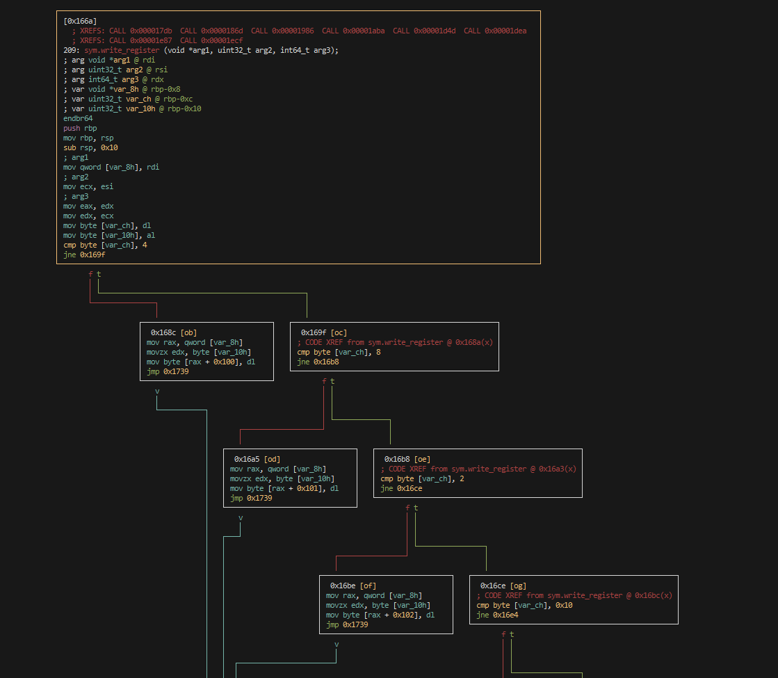
The control flow graph $G=<V,E>$ , where $V$ is a set of nodes (in our case, we have one node per basic block) and $E$ is a set of edges, where an edge is present if there is a jump between two basic blocks. Here is an example of CFG extracted with Radare2:

Instruction Normalization

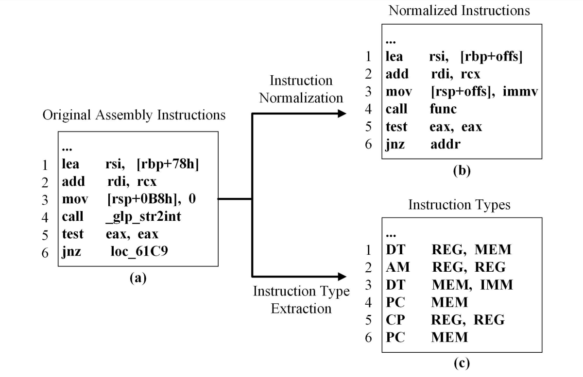
Binary code consists of a vast amount of different instructions, memory addresses, intermediate values, and address offsets. By naively taking these values and embedding them, we would end up with a lot of Out of Vocabulary (OOV) tokens. These are tokens that we have not seen during pretraining but are using during inference. Instruction normalization consists of a few simple rules where we replace tokens with special tokens:

immv for immediate values
addr for memory addresses
offs for address offsets
func for function names

Instruction Type Extraction

There is a distinction between binary code and natural text, as binary code follows a strict format. Binary consists of opcodes and operands, each playing a distinct role. To better capture these roles, we extract Instruction and Opcode Types from each basic block:

Opcode Type	Label	Example
Data transfer instruction	DT	mov, movq
Arithmetic instruction	AM	add, sub
Logical instruction	LG	and, or
Program control instruction	PC	jmp, call
Bit instruction	BI	shr, shl
Conditional move instruction	CM	cmova, cmovnb
Conditional set instruction	CS	setz, setle
Stack operation instruction	SO	push, pop
Data conversion instruction	DC	cvttsd2si, cvtsi2sd
Comparative instruction	CP	cmp, test

Operand Type	Label	Example
Register	REG	r0, rbx
Memory address	MEM	[rbx+offset], [rax]
Immediate value	IMM	01Ch, 0FFh

Semantic Learner

I already mentioned before, the Semantic Learner is just a BERT embedding model. BERT is usually trained with a Masked Token Prediction objective, and it is the case here as well, but we have an additional pretraining objective: Instruction Type Prediction. The output of the Semantic Learner consists of Node features, which are just the embeddings of basic blocks, and Edge features which are just concatenations of two Node embeddings that the edge connects.

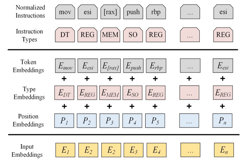
Instruction Type Prediction

If you read my BERT, CodeBERT and GraphCodeBERT summary, you should have a hunch how this will work. Essentially, after the last Attention/MLP layer of BERT, we end up with the contextual representation of a token, let’s call it $O$ . On top of $O$ , we are going to put an additional Multi Layer Perceptron (MLP) layer with softmax with the goal of predicting the instruction type for every instruction.

$p(instructionType|E_{mask}) = Softmax(MLP(O))$

The goal of this objective is to teach a model to reason about and determine different types of instructions that can be useful for downstream tasks.

Graph Learner

We have our CFG graph that we augmented with node and edge features to obtain the Augmented CFG (ACFG), which is just a triplet $G = <V,E,B>$ with $b_i \in B$ are the initial embeddings for a basic block belonging to $v_i \in V$ . Graph Matching network uses enhanced attention to compare two ACFGs $G_1 = <V_1, E_1, B_1>$ and $G_2=<V_2, E_2, B_2>$ to derive their embeddings and assess their similarity.

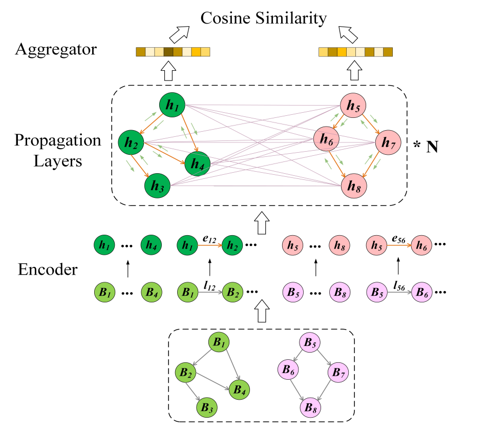
We can split Graph Learner into 3 parts:

Encoder
Propagation Layer
Aggregator

Encoder

Here we take the initial Node and Edge embeddings of an ACFG and pass each of them through a Linear Layer.

Propagation layer

Here we leverage the structure of the ACFG and we have a dual level attention mechanism that extracts information within a function (intra-function) and between functions (inter-function). Sounds extremely fancy but it is just message passing known from GNNs, where we use Graph Attention (GAT) but with the distinction that at the inter-function level we exchange information between nodes of different graphs.

Intra-function Attention

Here we focus on critical semantic details that are within each function.

$m_{j \rightarrow i} = f_{message}(h_i^{(t)}||h_j^{(t)}||e_{ij}), \forall(i,j) \in E$

$f_{message}$ is a multilayer perceptron that concatenates the inputs $h_i, h_j, e_{ij}$
$m_{j \rightarrow i}$ is the message from node j to node i

$a_{j \rightarrow i} = \frac{\exp(s_c(h_i^{(t)}, h_j^{(t)}))}{\sum_{j'} \exp(s_c(h_i^{(t)}, h_{j'}^{(t)}))}, j' \in N_i$

$N_i$ is the neighborhood of node i
$a_{j \rightarrow i}$ is the attention weight for information to be transmitted from j to i

$\gamma_i = \sum_j a_{j \rightarrow i}m_{j \rightarrow i}, j \in N_i$

$\gamma_i$ is aggregated information transmitted to node i from its neighborhood

Inter-Function Attention

Here we focus on capturing the semantic distinction between functions, enabling the model to detect homologous vulnerabilities across different but related functions. In the equations below, we compare nodes between 2 functions:

$a_{s \rightarrow i} = \frac{\exp(s_c(h_i^{(t)}, h_s^{(t)}))}{\sum_{s' \in V_2} \exp(s_c(h_i^{(t)}, h_{s'}^{(t)}))}$

$\mu_{s \rightarrow i} = a_{s \rightarrow i}(h_i^{(t)} - h_s^{(t)})$

$a_{s \rightarrow i}$ is the attention weight for information passed from node s of $G_2$ to node i of $G_1$ and $\mu_{s \rightarrow i}$ is the corresponding information

$\omega_i = \sum_{s \in V_2} \mu_{s \rightarrow i} = \sum_{s \in V_2} a_{s \rightarrow i}(h_i^{(t)} - h_s^{(t)}) = h_i^{(t)} - \sum_{s \in V_2} a_{s \rightarrow i}h_s^{(t)}$

we aggregate the passed information for node i from the closest node in the graph

$h_i^{(t+1)} = f_{update}(h_i^{(t)}, \gamma_i|| \omega_i)$

we then process the nodes with Gated Recurrent Network (GRU)
now we run it for T rounds and combine the individual node information into a single embedding:

$h_G = MLP_G(\sum_{i \in V} \sigma(MLP_{gate}(h_i^{(T)}) \odot MLP(h_i^{(T)})))$

here it is worth noting that this creates quite an information explosion, since we do pairwise comparison between so many functions that we use

Aggregator

This is the last part, remember the goal of GMN+ is to determine if two functions are homologous! To enforce similarity and dissimilarity we use Contrastive Learning to push the embeddings of similar functions together and dissimilar functions apart.

$L_G = \log(1 + e^{\cos(h_{G_1},h_{G_3})} - e^{\cos(h_{G_1},h_{G_2})})$

$G_1, G_2$ are homologous and $G_1, G_3$ are not

Remarks

There is an obvious issue here, inside the Propagation Layer we do quite a lot of message passing between individual nodes, this can easily get out of hand if we are working with a huge function (or multiple huge functions).

Experiments

Long story short, GMN+ achieves state-of-the-art performance in terms of binary function similarity detection and is also able to uncover vulnerabilities in real-life repositories of:

sqlite3
glpk
xml

Similarity Detection

Here we compile with GCC targeting ARM, MIPS and X86 with all 3 optimization levels O1, O2 and O3.

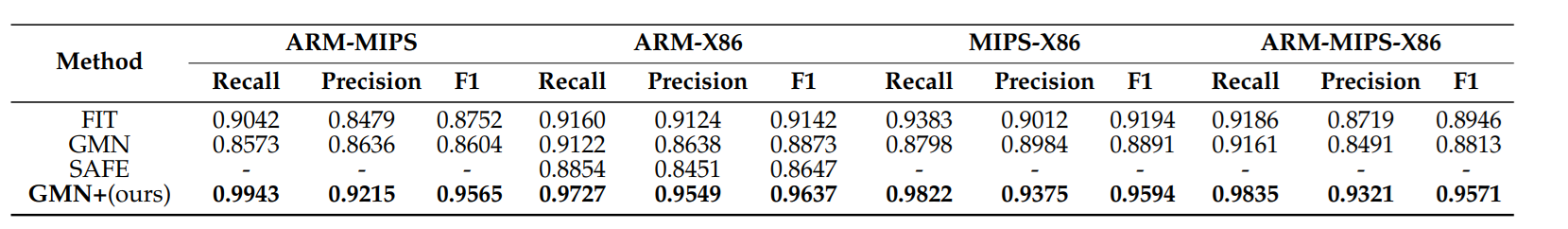
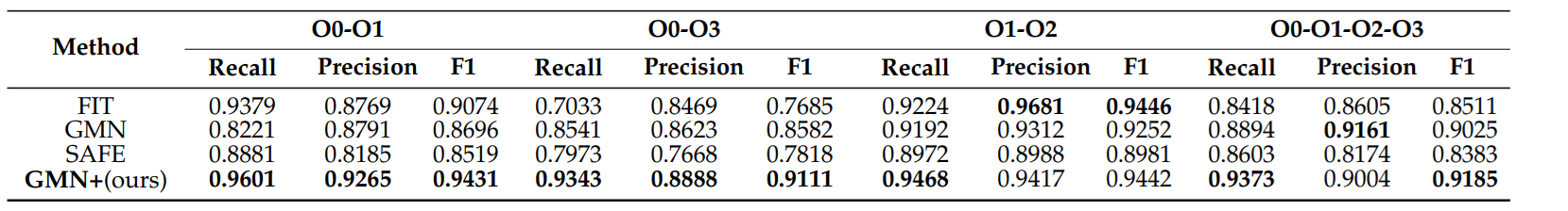
Why is this benchmark important? First, if you are working with a stripped binary, you have no access to symbols, having a library of common utility functions can enormously help with reverse engineering.

Vulnerability Detection

Again we can see that GMN+ is able to find more real-world vulnerabilities than other methods.

However, here is a catch: we need to compare functions against a set of functions that are known to be vulnerable, making it hard to use in practice.

Final Remarks

GMN+ is an exciting research direction. By leveraging past vulnerabilities, we focus on finding future vulnerabilities that are similar. This concept is simple; however, for practice, it requires building a huge database of vulnerable functions. Sure there are some datasets, but as multiple research papers point out, they often have toy examples or are outdated. And at last, there is the aspect of exploitability of a vulnerability, which is a task of multiple orders of magnitude harder, but for the field of vulnerability research way more important.